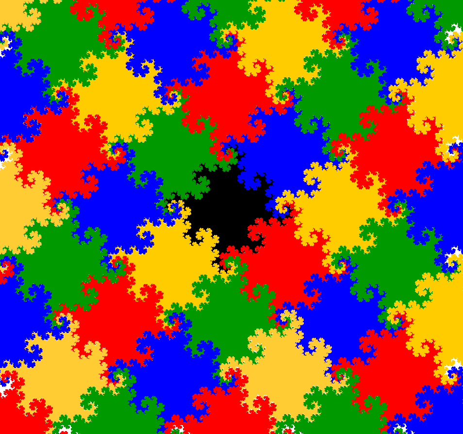

Heighway Dragon Tiling
Music: The Morning Sun by Ethereal 88 | https://ethereal88.bandcamp.com
Version 1
via squares
and IFS
We consider the Heighway dragon as constructed by an iterated function system with an initial segment of length 1. An IFS for this construction is given by the following.
where \(r = \frac{1}{{\sqrt 2 }}\). At each iteration, scale the current figure by \(r = \frac{1}{{\sqrt 2 }}\) and rotate by 45 around the origin. This is function \(f_1\). Then make a copy of this figure and rotate it by 90° around the point (1/2,1/2). This will give an equivalent result as the function \(f_2\).
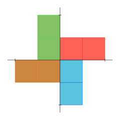
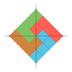
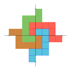
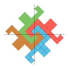
Starting with any compact set, iterations of that set using the two functions in this IFS will always converge to the Heighway dragon. We can start with a square \(S_0\) whose diagonal is the initial segment of length 1. let \(S_n\) denote the sequence of iterations of \(S_0\), i.e. \({S_{n+1} = f_1(S_n)\cup f_2(S_n)}\). The sets \(S_n\) for \(n = 0,1,2,3,4\) are shown below.
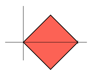
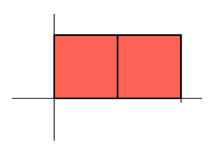
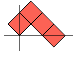
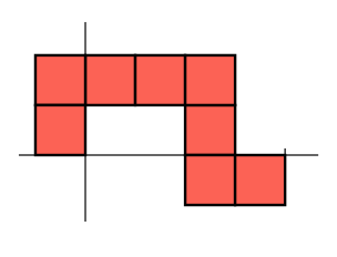
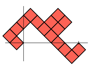
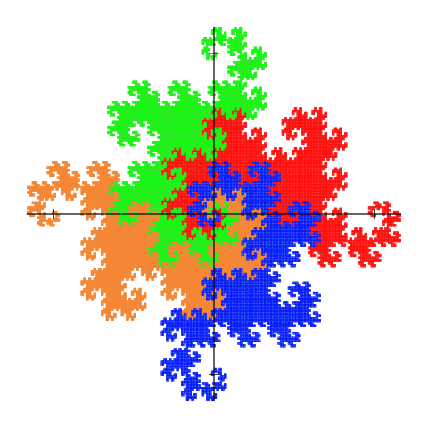
Each of these iterations can form a tile by rotating a copy of each by 90°, 180°, and 270° around the origin. The copies are disjoint up to measure 0, i.e. they do not overlap except along the boundaries. (We will always use "disjoint" to mean "disjoint up to measure 0".)
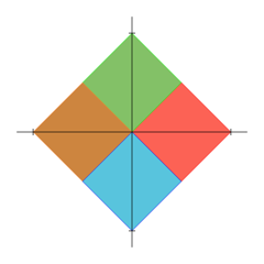
Convergence
Video
Let \(T_n\) be the tile formed this way from the set \(S_n\). Since the sets \(S_n\) converge to the Heighway dragon, the sets \(T_n\) converge in the Hausdorff metric to \(H_4\), four disjoint copies of the Heighway dragon rotated 0°, 90°, 180°, and 270° around the origin.
Each set \(T_n\) can form a lattice tiling of the plane using the lattice shown below that is formed by the vectors \(\mathbf{v_1} = (1,1)\) and \(\mathbf{v_2} = (1,-1)\). Let \(\Lambda = \{k_1\mathbf{v_1} + k_2\mathbf{v_2}: k_1, k_2 \in \mathbb{Z} \}\) be the corresponding lattice points. These form a discrete translation set for the tiling. This means that \(\Lambda\) is a subset of the plane such that for every bounded region of the plane, there are only finitely many points of \(\Lambda\) inside the region, and \[\bigcup_{\lambda \in \Lambda} (T_n + \lambda) = \mathbb{R}^2.\] This condition means that if we take every point \(\lambda \in \Lambda\) and shift \(T_n\) by that vector, the collection of all such translated copies covers the entire plane. In other words, every point of \(\mathbb{R}^2\) lies in a translate of \(T_n\).
Click on each of the buttons to the left to see a partial tiling for the first 9 iterations. At this size and resolution, you will not see much difference past \(n = 9\).
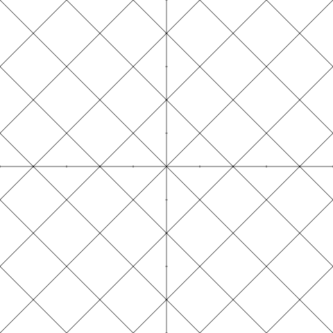
Since each of the sets \(T_n\) tiles the plane, and the sets \(T_n\) converge to the \(H_4\), the four copies of the Heighway dragon, then \(H_4\) will also tile the plane. Here's why.
Suppose \(z\) is a point in the plane. For every \(n\), there is a point \(\lambda_n\) in \(\Lambda\) such that \(z\) is in the set \(T_n + \lambda_n\). Now all the sets \(T_n\) and the point \(z\) lie inside a circle of a sufficiently large radius. This means that the collection \((\lambda_n)\) will lie in a bounded region. Since \(\Lambda\) is a discrete translation set, only a finite number of members of \(\Lambda\) are in that bounded region. Therefore there must be a subsequence \((\lambda_{n_k})\) all of whose terms are equal to a constant \(\lambda\). Now let \(\varepsilon > 0\). Since the sets \(T_{n_k}\) converge to \(H_4\) in the Hausdorff metric, there is an integer \(M\) such that \(T_{n_k} \subset N_\varepsilon(H_4)\) for all \(n_k \ge M\), where \(N_\varepsilon(H_4)\) is the \(\varepsilon\)-neighborhood of \(H_4\), i.e. all the points within a distance \(\varepsilon\) of \(H_4\). But then \(T_{n_k}+\lambda \subset N_\varepsilon(H_4+\lambda)\) for all \(n_k \ge M\). Therefore \(z \in N_\varepsilon(H_4+\lambda)\) for all \(\varepsilon > 0\), so we must actually have \(z \in H_4+\lambda\). Thus \(\displaystyle \bigcup_{\lambda \in \Lambda}(H_4+\lambda) = \mathbb{R}^2\).
Version 2
via L-system
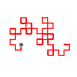
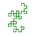
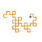
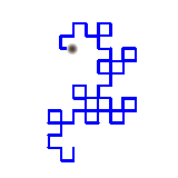
The iteration of the L-system generates the "dragon curve". The individual line segments never cross. Now take the nth iterate in the construction and draw a square lattice on the plane of size \({(\frac{1}{{\sqrt 2 }})^n}\), where n is even (if you want to do this with any n, it would be necessary to rotate the lattice by 45° and scale the grid by \({(\frac{1}{{\sqrt 2 }})}\)). Starting with an initial line of length 1, we can draw the segments in the dragon construction so that the corners always occur at these lattice points in the plane. Harter was the first to show that copies of the dragon could be fitted together to cover all lattice points. For example, shown below is the 6th iterate (in red) and three copies, each rotated by a multiple of 90°. The dot indicates the beginning of the curve (the tail). The lattice is of grid size 1/8.
Geogebra
Animation
Now join each of the curves tail to tail by clicking on the buttons to the left in sequence.

The image below shows four copies of the 8th iterate of the Heighway dragon. Click on the play button to see an animation of the iterates starting at the beginning of each curve that demonstrates how each of the four different dragons fit together to tile the plane. The three buttons labeled slower, normal, and faster will adjust the drawing speed.
Higher order iterates would continue to cover lattice points on a smaller scale [Example with 10 iterations (pdf)]. In the limit, four copies of the dragon would exactly nestle together as you can demonstrate by clicking on the following buttons in sequence.

The four pieces form an image with 90° rotational symmetry. The entire plane can be covered by copies of this combined image [Example].
See the four rotated copies of the Heighway dragon done in counted cross-stitch.